Implied Volatility, Standard Deviation and Expected Price Moves
No matter what type of security or financial instrument one might be trading, the expected price range of the underlying is typically a critical factor in determining how to capitalize upon a given opportunity.
While many option traders understand and use implied volatility in their decision-making process, fewer of them delve into standard deviation. The term itself sounds a bit “mathy,” which may be a big reason why it so often gets overlooked.
However, given the close, intertwined relationship between implied volatility and standard deviation, it’s likely a strong understanding of both concepts will assist traders in better assessing the relative attractiveness of ongoing opportunities.
The main reason standard deviation is so critical is because it can provide traders with a reference point for the market’s expected price range for a given underlying, and how likely it is for that underlying to ultimately land in said range.
Implied volatility itself is defined as a one standard deviation annual move. On top of that, a one standard deviation move encompasses the range a stock should trade in 68.2% of the time. That information on its own is pretty powerful.
For example, imagine hypothetical stock XYZ is trading for $200 with an implied volatility of 10%. That means XYZ has an implied 68.2% chance of trading between $180 and $220 during a one year timeframe ($200 x 0.10 = +/-$20).
Additionally, that implies there’s a 95.4% chance that XYZ will trade between $160 and $240, and a 99.7% chance that it will trade between $140 and $260 over a one year timeframe.
These probabilities are derived from a statistical function known as a probability distribution. Probability distributions, often presented as “bell curves,” describe all the possible values and likelihoods that a random variable can take within a given range.
Stock prices have historically exhibited log-normal behavior, which in layman’s terms means they are well-suited for probability distributions.
While the calculation for standard deviation looks a little messy at first glance, it’s actually fairly straight-forward. As shown in the slide below, the calculation for standard deviation incorporates implied volatility and the time until expiration:
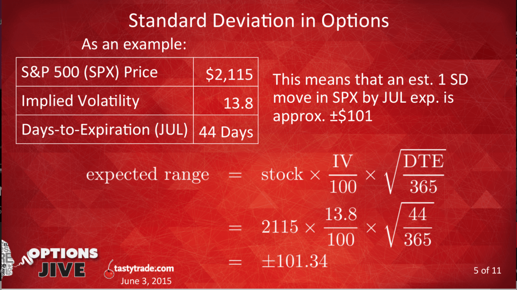
Based on the above, it’s now a little easier to visualize how changes in implied volatility (as well as time until expiration) might affect the expected range for a given underlying.
For example, when implied volatility increases, the range of prices encompassed by a one standard deviation move also gets wider. This is illustrated in the chart below:
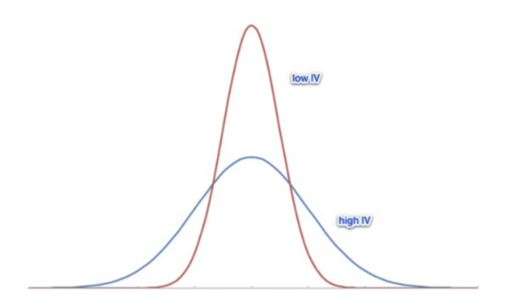
Periods of low implied volatility therefore imply tight ranges for an underlying, while rising implied volatility provides wider ranges in which an underlying could theoretically trade.
Importantly, rising implied volatility also translates to higher premiums paid/received when buying/selling options in the associated underlying.
Revisiting the earlier example, if implied volatility were to increase from 10% to 25% in sample stock XYZ, the new probability distribution would be:
- 1 standard deviation move (68.2%) between $150 and $250
- 2 standard deviation move (95.4%) between $100 and $300
- 3 standard deviation move (99.7%) between $50 and $350
Given that a 10% implied volatility for underlying XYZ equated to a 1 standard deviation move between $180 and $220, one can see just how drastically expectations for movement in this hypothetical underlying have shifted in a rising volatility environment.
In practice one can also see how changes in implied volatility and standard deviation might also create a more attractive potential opportunity for an options trader. When implied volatility was only 10%, a trader seeking to sell a one standard deviation strangle would have been targeting the $180 and $220 strikes.
However, due to the widening of expectations in the potential movement of XYZ, an implied volatility of 25% means that the associated 1 standard deviation strangle would now fall to the $150 and $250 strikes, respectively.
Consequently, in high volatility environments, when expectations for movement are expanding, short volatility traders have a choice available to them:
- Sell strikes that are closer to at-the-money (ATM), with higher credits received, but with lower probability of profit (POP)
- Sell strikes that are further from at-the-money (ATM), with slightly lower credits received, but with higher probability of profit (POP)
To review the risk-reward ramifications of these two choices, traders may want to review a previous installment of Market Measures on the tastytrade financial network.
The information presented on this episode stems from internal tastytrade research which leverages historical market data and helps illustrate the relative advantages and disadvantages of the two trading approaches. A comprehensive review of this material should better equip traders to evaluate such decisions going forward.To learn more about implied volatility and standard deviation, additional information is also available in the tastytrade LEARN CENTER.
Sage Anderson is a pseudonym. The contributor has an extensive background in trading equity derivatives and managing volatility-based portfolios as a former prop trading firm employee. The contributor is not an employee of luckbox, tastytrade or any affiliated companies. Readers can direct questions about any of the topics covered in this blog post, or any other trading-related subject, to support@luckboxmagazine.com.