The 2022 trading year has been somewhat unusual because investors and traders have been dealing with persistent bear market conditions.

Since the end of the Great Recession, bear markets have been somewhat rare, which means that most market participants these days are likely tuned into booking profits in bull markets. 

However, bear markets offer plenty of opportunities for savvy market participants, which means that an active approach can still be fruitful at this time, as well. And this goes for stock traders and options traders alike.

Trading Stocks in a Bearish Environment

Investors and traders with an overall long bias have felt the hurt in 2022.

At the end of August, Federal Reserve Chairman Jerome Powell kicked off a fresh round of selling in the stock market stemming from his hawkish speech in Jackson Hole, Wyoming.

Since that speech on Aug. 26, the S&P 500 and the Nasdaq 100 are down 6.5% and 8%, respectively.

During 2020, the stock market also experienced a sharp correction, but the stock market rebounded that year in rapid fashion as a slew of market participants “bought the dip.” In 2022, bear market conditions have been more persistent, and buying the dip hasn’t been as effective.  

“Buy the dip” refers to a trading and investing approach that involves purchasing an asset (or group of assets) after a significant drop in price. For example, if a trader or investor liked Apple (AAPL) at $150/share, wouldn’t he or she like it even more if it dropped to $130/share?

While the approach has been around for a long time, buying the dip gained newfound fame in 2020. Since then, dip buying has seemingly gained even more traction in the markets as more and more market participants have jumped on board. And a close cousin of buying the dip is known as “dollar cost averaging.”

Dollar-cost averaging refers to the practice of systematically investing into a security or asset over a period of time, regardless of price. So, an investor looking to deploy $100,000 into a given stock might start with $20,000, and then deploy an additional $20,000 four more times over the course of the next several weeks/months/years to complete the full $100,000 investment. 

This approach can be executed at regular intervals—once a month or once a quarter, for example—or at irregular intervals, depending on the vision of the investor or trader in question. 

Considering that securities tend to fluctuate in value over time, one can see how dollar-cost averaging can reduce the overall impact of volatility on the price of the target asset. That’s because the price paid for the security will vary each time a periodic investment is made.

Looking at an example, consider an investor with a long-term bullish bias that holds a long stock position in Nvidia (NVDA). Now imagine this hypothetical investor purchased 100 shares of NVDA for $230/share back in March of 2022.

Since that time, NVDA has dropped down to roughly $130/share. The investor has taken a considerable loss in this position—losing roughly $10,000, or 43% of the original investment. However, if the investor is still bullish on NVDA’s long-term prospects, he or she could potentially increase the size of his or her stake in NVDA at a more attractive entry point.

Assuming the investor purchases another 100 shares at the current price of $130/share, one can then calculate the cost basis for the overall NVDA position. To calculate the cost basis, one simply adds together the cost of each individual entry point, and divides it by the total number of shares. 

For example, entry point A would equate to $23,000 (100 shares x $230/share) and entry point B would equate to $13,000 (100 shares x $130/share). To calculate the cost basis, simply add together $23,000 + $13,000 and then divide it by 200 shares, which equates to $180/share ($36,000/200 shares = $180/share).

That new cost basis—utilizing a dollar-cost averaging approach—is a lot more attractive than the original cost basis, which was $230/share.

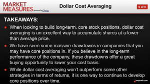
This example helps illustrate how market participants can use dollar-cost averaging in the current environment to capitalize on weakness in the markets, with the intent of profiting over the longer term.

Trading Options in a Bearish Environment

Just like in the stock market, investors and traders can leverage bear market conditions to capitalize on opportunities in the options market.

Of course, the particular strategy (or strategies) utilized in the options market will depend on one’s unique market outlook and risk profile. 

An investor or trader attempting to play a rebound in the stock market might sell a put, or sell a put spread. Alternatively, an investor or trader that expects the market to move lower might buy a naked put, or deploy a bear put spread.

Bullish Outlook, Bull Put Spread

Bull put spreads are often utilized by investors and traders that expect a moderate rise in the price of the underlying asset. Bull put spreads are a type of vertical spread. 

A vertical spread is constructed using one long option and one short option. In a vertical, both options should be of the same type and in the same expiration month, but of different strike prices.

Accordingly, a vertical consists of a long call and a short call, or a long put and a short put. Moreover, one of the options in the spread will be in-the-money (ITM), while the other will be out-of-the-money (OTM). The latter, OTM, serves as the “wing” of the position. 

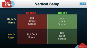
Verticals are always executed in 1-to-1 fashion, or the same number of contracts on each leg of the trade. Therefore, a vertical spread can be deployed in four different ways, as illustrated in the graphic below. 

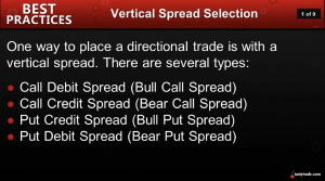
As a reminder, “credit spreads” refer to positions in which the trader collects premium when taking into account the combined cost of the spread, whereas “debit spreads” refer to positions in which the trader outlays premium when taking into account the combined cost of the spread.

Generally speaking, debit spreads are long premium positions that benefit from rising implied volatility environments, while credit spreads are short premium positions that benefit from declining implied volatility environments. 

In the case of the put credit vertical spread, this position hinges on selling an ITM put, while purchasing another lower strike put for protection.

The bull put spread looks to take advantage of an increase in price in the underlying asset before expiration. Time decay and decreased implied volatility will also benefit the bull put spread. 

Since this is a credit spread and a “defined risk” position, the maximum gain is restricted to the net premium received for the position, while the maximum loss is equal to the difference in the strike prices of the puts less the net premium received.

To learn more about bull put credit spreads, check out this installment of Options Trading Concepts on the tastytrade financial network. 

Bearish Outlook, Bear Put Spread

Investors and traders with a bearish view on the stock market can also express that outlook using options. 

Purchasing a naked put is obviously one clear choice available to bearish market participants. But one should keep in mind that in a bearish environment, implied volatility (i.e. the price of an option) is elevated. That means puts are more expensive as compared to a “normal” or “complacent” market environment. 

To help offset the cost of a naked put, investors and traders can consider another form of vertical spread—the put debit vertical spread. This position is commonly referred to as a “bear put spread.”

Using this approach, one purchases an ITM put, while simultaneously selling a lower strike OTM put in the same expiration period. 

The total cost of a put debit vertical spread is calculated by taking the long premium less the short premium, which in sum is referred to as the total debit. If the underlying fails to drop in price, the trader will have saved themself valuable capital via the short OTM put.

That’s one reason the bear put spread may be preferable to a naked put. 

Debit vertical spreads are “defined risk” positions, which means the maximum loss is restricted to the net premium paid for the position, while the maximum profit is equal to the difference in the strike prices of the puts less than the net premium paid to put on the position.

To learn more about vertical spreads, check out this installment of Tasty Bites on the tastytrade financial network. For more on dollar-cost averaging, watch this episode of Market Measures.

For daily updates on everything moving the markets, tune into TASTYTRADE LIVE—weekdays from 7 a.m. to 4 p.m. CDT.

Sage Anderson is a pseudonym. He’s an experienced trader of equity derivatives and has managed volatility-based portfolios as a former prop trading firm employee. He’s not an employee of Luckbox, tastytrade or any affiliated companies. Readers can direct questions about this blog or other trading-related subjects, to support@luckboxmagazine.com.