Understanding the Black-Scholes Options Pricing Model
The Black-Scholes model, which was first devised by Fischer Black and Myron Scholes in 1973, has become an ubiquitous options pricing model because it largely relies on easily observable financial data.
When investors and traders pull up a quote, what’s observed is the current market price of that asset. But what’s not observed is that market prices are usually underpinned by a wide range of asset pricing models.
For example, when ascertaining the “fair value” of a given stock, an investor or trader might use a pricing model such as the Discounted Cash Flow Model (DCF), the Dividend Discount Model (DDM), or the Capital Asset Pricing Model (CAPM)—among many others.
No matter the pricing model selected, the output produces a theoretical fair value. But there’s no guarantee that the theoretical value produced by a given pricing model will match the value observed in the market.
That’s because models often rely on a variety of assumptions, many of which may be incorrect, unknown or both.
For example, an investor using the DCF model to value Apple (AAPL) stock may have used sales and earnings projections that are deemed too conservative by the market. Varying assumptions such as this help explain why an investor’s theoretical price for Apple stock might be different from the actual price observed in the market.
And that’s not a bad thing, because discrepancies in valuations technically produce opportunities for inventors and traders. That’s where the risk/reward dynamic of the market comes into play.
Of course, for an emerging asset class such as cryptocurrencies, there’s far less agreement on how such digital assets should be valued. Pricing models do exist for the cryptocurrency sector, but the best model(s) may only be known or understood by a select few.
At this time there’s no method for pricing cryptocurrencies that’s (as yet) universally agreed upon.
Notably, the equity options market lies at the other end of the pricing model spectrum. Virtually all market participants in the stock options market use the Black-Scholes model—or an adjusted version—to price options.
The Black-Scholes Formula is a mathematical equation that was first published by Fischer Black and Myron Scholes in 1973. The formula, known widely as the “Black-Scholes model,” is a partial differential equation that estimates the value of an option over time.
The Black-Scholes model incorporates probability theory to estimate the future value of a stock using the historical movement of the stock as a predictive component. This concept is encapsulated in the term “volatility.”
Volatility is usually described according to three different classifications: historical volatility, implied volatility and future volatility.
Historical volatility measures the variation of price in an underlying stock over a distinct period of time in the past. Historical volatility is often referred to as “actual volatility,” because it can be directly observed using historical data.
Implied volatility, on the other hand, is derived from the market value of an option price and expressed in volatility terms (as opposed to dollars and cents). Future volatility is the greatest unknown in options pricing and trading because it represents the future variation in the price of a stock, which is obviously unknown.
Generally speaking, the Black-Scholes model uses five basic inputs in order to calculate a theoretical value for an option, including volatility:
1. Strike price
2. Time to expiration
3. Current stock price
4. Risk-free rate
5. Volatility of the stock
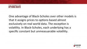
The first four variables listed above are observable, and the model’s reliance on easily accessible data is a big reason it has become so ubiquitous.
The fifth input is a key reason that the model produces a theoretical value that may not mirror the exact price trading in the market. The Black-Scholes model assumes that volatility is constant, but as most options traders are well aware, that simply isn’t the case.
Volatility fluctuates over time, which is why opportunity exists in the options market.
Without getting too caught up in the exact mechanics of the Black-Scholes equation, the important thing to understand is that there exists a standard equation that serves as the foundation of pricing for the options world.
And while the Black-Scholes model was the original formula for calculating the theoretical price of an option, other members of the academic and private-sector communities have created adjusted versions of the Black-Scholes model which are also now in use—not only in the options market, but also in the futures and foreign currency markets.
To learn more about the mathematics underpinning the Black-Scholes model, readers may want to review a recent episode of The Skinny on Options Math on the tastytrade financial network.
Readers interested in learning more about the mathematics behind options, and other tradable products, may also want to explore The Skinny on Options Math episode archives when scheduling allows.
Content in this series focuses on, but isn’t limited to, broad-based discussions on the Black-Scholes model and its variables, adjusted versions of the model, data used in the model—as well as other terms/concepts/models critical to the mathematics that underpin trading and investing.
For updates on everything moving the markets, readers can also tune into TASTYTRADE LIVE—weekdays from 7 a.m. to 4 p.m. CST.
Sage Anderson is a pseudonym. He’s an experienced trader of equity derivatives and has managed volatility-based portfolios as a former prop trading firm employee. He’s not an employee of Luckbox, tastytrade or any affiliated companies. Readers can direct questions about this blog or other trading-related subjects, to support@luckboxmagazine.com.